

Linear programs are problems that can be expressed as
\[\min_{x}c^{\top}x\text{ subject to }Ax=b, x\geq0\]where \(x\in\mathbb{R}^{n}\) are variables, \(A\in\mathbb{R}^{m\times n}\)
is the constraints matrix, \(b\in\mathbb{R}^{m}\)
and \(c\in\mathbb{R}^{n}\) are the coefficients. Many practical problems
in both operations research and computer science can be expressed
or approximated as linear programs. Examples include shortest path,
maximum flow, multi commodity flow, bipartite matching, scheduling
problems, personnel/inventory management, etc. In this blog, we will
discuss the recent result of Michael Cohen, Zhao Song and me about
an nearly ‘‘optimal’’ algorithm for linear programs.
Background
For an arbitrary linear program \(\min_{Ax=b,x\geq0}c^{\top}x\) with \(n\) variables and \(d\) constraints, the fastest algorithm [LS15] takes \(O^{*}(\sqrt{d}\cdot\mathrm{nnz}(A)+d^{2.5})\) where \(\mathrm{nnz}(A)\) is the number of non-zeros in \(A\), \(O^{*}\) hides all \(n^{o(1)}\) and \(\log^{O(1)}(1/\epsilon)\) factors, and \(\epsilon\) is the target accuracy.
For the generic case \(d=\Omega(n)\) we focus in this blog, the current fastest runtime is dominated by \(O^{*}(n^{2.5})\). This runtime has not be been improved since the result by Vaidya on 1989. The \(n^{2.5}\) bound originated from two factors: the cost per iteration \(n^{2}\) and the number of iterations \(\sqrt{n}\). The \(n^{2}\) cost per iteration looks optimal because this is the cost to compute \(Ax\) for a dense \(A\). Therefore, many efforts have been focused on decreasing the number of iterations while maintaining the cost per iteration. As for many important linear programs (and convex programs), the number of iterations has been decreased, including maximum flow [M16], minimum cost flow [CMSV17], geometric median [CLMPS16], matrix scaling and balancing [CMTV17], and \(\ell_p\) regression [BCLL18]. Unfortunately, beating \(\sqrt{n}\) iterations (or \(\sqrt{d}\) when \(d\ll n\)) for the general case remains one of the biggest open problems in optimization.
In this blog, we will discuss how to avoid this open problem and develop a stochastic central path method that has a runtime of
\[O^{*}(n^{\omega}+n^{2+1/3})=O^{*}(n^{\omega})\]where \(\omega\sim2.37286\) is the exponent of matrix multiplication [CW87, Wil12, DS13, Le14]. This achieves the natural barrier for solving linear programs because linear system is a special case of linear program and that the currently fastest way to solve general linear systems involves matrix multiplication.
Main Result
Given a linear program \(\min_{Ax=b,x\geq0}c^{\top}x\) with no redundant constraints. Assume that the polytope has diameter \(R\) in \(\ell_{1}\) norm, namely, for any \(x\geq0\) with \(Ax=b\), we have \(\|x\|_{1}\leq R\). Then, for any \(0<\delta\leq1\), we can find \(x\geq0\) such that \(c^{\top}x \leq\min_{Ax=b,x\geq0}c^{\top}x+\delta\cdot\|c\|_{\infty}R\)
and
\[\|Ax-b\|_{1} \leq\delta\cdot\left(R\sum_{i,j} | A_{i,j} |+\|b\|_{1}\right)\]in expected time
\[\left(n^{\omega+o(1)}+n^{2.5-\alpha/2+o(1)}+n^{2+1/6+o(1)}\right)\cdot\log(\frac{n}{\delta})\]where \(\omega\) is the exponent of matrix multiplication, \(\alpha\) is the dual exponent of matrix multiplication, defined by the supremum among all \(a\geq 0\) such that it takes \(n^{2+o(1)}\) time to multiply an \(n \times n\) matrix by an \(n \times n^a\) matrix.
Central Path Method
Our algorithm relies on two new ingredients: stochastic central path and projection maintenance. The central path method consider the linear program
\[\min_{Ax=b,x\geq0}c^{\top}x\quad\text{(primal)}\quad\text{and}\quad\max_{A^{\top}y\leq c}b^{\top}y\quad\text{(dual)}\]with \(A \in \mathbb{R}^{d \times n}\). Any solution of the linear program satisfies the following optimality conditions:
\[\begin{align} x_{i}s_{i} & =0\text{ for all }i,\\ Ax & =b,\\ A^{\top}y+s & =c,\\ x_{i},s_{i} & \geq0\text{ for all }i. \end{align}\]We call \((x,s,y)\) feasible if it satisfies the last three equations above. For any feasible \((x,s,y)\), the duality gap is \(\sum_{i}x_{i}s_{i}\). The central path method find a solution of the linear program by following the central path which uniformly decrease the duality gap. The central path \((x_{t},s_{t},y_{t})\in\mathbb{R}^{n+n+d}\) is a path parameterized by \(t\) and defined by
\[\begin{align} x_{t,i}s_{t,i} & =t\text{ for all }i,\\ Ax_{t} & =b,\\ A^{\top}y_{t}+s_{t} & =c,\\ x_{t,i},s_{t,i} & \geq0\text{ for all }i. \end{align}\]It is known [YTM94] how to transform linear programs by adding \(O(n)\) many variables and constraints so that:
- The optimal solution remains the same.
- The central path at \(t=1\) is near \((1_n,1_n,0_d)\) where \(1_n\) and \(0_d\) are all \(1\) and all \(0\) vectors with appropriate lengths.
- It is easy to covert an approximate solution of the transformed program to the original one.
Therefore, it suffices to show how to move gradually \((x_{1},s_{1},y_{1})\) to \((x_{t},s_{t},y_{t})\) for small enough \(t\).

Short Step Central Path Method
The short step central path method maintains \(x_{i}s_{i}=\mu_{i}\) for some vector \(\mu\) such that
\[\sum_i (\mu_i - t)^2 = O(t^2)\]for some scalar \(t > 0\).
To move from \(\mu\) to \(\mu+\delta_{\mu}\) approximately, we approximate the term \((x+\delta_{x})_i(s+\delta_{s})_i\) by \(x_i s_i+x_i\delta_{s,i}+s_i\delta_{x,i}\) and obtain the following system #1:
\[\begin{align} X\delta_{s}+S\delta_{x} & =\delta_{\mu},\notag\\ A\delta_{x} & =0,\label{eq:delta_x_s_y_mu}\\ A^{\top}\delta_{y}+\delta_{s} & =0,\notag \end{align}\]where \(X=\mathrm{diag}(x)\) and \(S=\mathrm{diag}(s)\). This equation is the linear approximation of the original goal (moving from \(\mu\) to \(\mu+\delta_{\mu}\)), and that the step is explicitly given by the formula #2
\[\delta_{x}=\frac{X}{\sqrt{XS}}(I-P)\frac{1}{\sqrt{XS}}\delta_{\mu}\text{ and }\delta_{s}=\frac{S}{\sqrt{XS}}P\frac{1}{\sqrt{XS}}\delta_{\mu}\]where \(P=\sqrt{\frac{X}{S}}A^{\top}\left(A\frac{X}{S}A^{\top}\right)^{-1}A\sqrt{\frac{X}{S}}\) is an orthogonal projection and the formulas \(\frac{X}{\sqrt{XS}}, \frac{X}{S}, \cdots\) are the diagonal matrices of the corresponding vectors.
A standard choice of \(\delta_{\mu,i}\) is \(- t/\sqrt{n}\) for all \(i\) and this requires \(\tilde{O}(\sqrt{n})\) iterations to converge. Combining this with the inverse maintenance technique [V87], this gives a total runtime of \(n^{2.5}\). We remark that \(\sum_i (\mu_i - t)^2 = O(t^2)\) is an invariant of the algorithm and the progress is measured by \(t\) because the duality gap is roughly \(n t\).
Stochastic Central Path Method
Now, we discuss how to modify the short step central path to decrease the cost per iteration to roughly \(n^{\omega-\frac{1}{2}}\). Since our goal is to implement a central path method in sub-quadratic time per iteration, we even do not have the budget to compute \(Ax\) every iterations. Therefore, instead of maintaining \(\left(A\frac{X}{S}A^{\top}\right)^{-1}\) shown in previous papers, we will study the problem of maintaining a projection matrix
\[P=\sqrt{\frac{X}{S}}A^{\top}\left(A\frac{X}{S}A^{\top}\right)^{-1}A\sqrt{\frac{X}{S}}\]due to the formula #2 of \(\delta_x\) and \(\delta_s\).
However, even if the projection matrix \(P\) is given explicitly for free, it is difficult to multiply the dense projection matrix with a dense vector \(\delta_\mu\) in time \(o(n^{2})\). To avoid moving along a dense \(\delta_{\mu}\), we move along an \(O(k)\) sparse direction \(\tilde{\delta}_{\mu}\) defined by
\[\begin{align} \tilde{\delta}_{\mu,i}=\begin{cases} \delta_{\mu,i}/p_{i} , & \text{with probability }p_{i}:= k\cdot\left(\frac{\delta_{\mu,i}^{2}}{ \sum_{l}\delta_{\mu,l}^{2} }+\frac{1}{n}\right);\\ 0 , & \text{else}. \end{cases}\label{eq:tilde_delta_mu} \end{align}\]The sparse direction is defined so that we are moving in the same direction in expectation (\(\mathbb{E} [ \tilde{\delta}_{\mu,i} ] = \delta_{\mu,i}\)) and that the direction has as small variance as possible (\(\mathbb{E} [ \tilde{\delta}_{\mu,i}^{2} ] \leq\frac{\sum_{i}\delta_{\mu,i}^{2}}{k}\)). If the projection matrix is given explicitly, we can apply the projection matrix on \(\tilde{\delta}_{\mu}\) in time \(O(nk)\). Picking \(k\sim\sqrt{n}\), the total cost of projection vector multiplications is about \(n^{2}\).
During the whole algorithm, we maintain a projection matrix
\[\overline{P}=\sqrt{\frac{\overline{X}}{\overline{S}}}A^{\top}\left(A\frac{\overline{X}}{\overline{S}}A^{\top}\right)^{-1}A\sqrt{\frac{\overline{X}}{\overline{S}}}\]for vectors \(\overline{x}\) and \(\overline{s}\) such that \(\overline{x}_{i}=\Theta(x_{i})\) and \(\overline{s}=\Theta(s_{i})\) for all \(i\). Since we maintain the projection at a nearby point \((\overline{x}, \overline{s})\), our stochastic step \(x\leftarrow x+\tilde{\delta}_{x}\), \(s\leftarrow s+\tilde{\delta}_{s}\) and \(y\leftarrow y+ \tilde{\delta}_{y}\) are defined by
\[\begin{align} \overline{X}\tilde{\delta}_{s}+\overline{S}\tilde{\delta}_{x} & =\tilde{\delta}_{\mu},\notag\\ A \tilde{\delta}_{x} & =0,\label{eq:tilde_delta_x_s_y_mu}\\ A^{\top}\tilde{\delta}_{y}+ \tilde{\delta}_{s} & =0,\notag \end{align}\]which is different from (system #1)[#delta_x_s_y_mu] on both sides of the first equation. Similar to formula #2, one can show that
\[\tilde{\delta}_{x}=\frac{\overline{X}}{\sqrt{\overline{X}\overline{S}}}(I-\overline{P})\frac{1}{\sqrt{\overline{X}\overline{S}}}\tilde{\delta}_{\mu}\text{ and }\tilde{\delta}_{s}=\frac{\overline{S}}{\sqrt{\overline{X}S}}\overline{P}\frac{1}{\sqrt{\overline{X}\overline{S}}}\tilde{\delta}_{\mu}.\]The previously fastest algorithm involves maintaining the matrix inverse \(( A \frac{X}{S} A^\top )^{-1}\) using subspace embedding techniques [Sar06,CW13,NN13] and leverage score sampling [SS11]. In the next section, we will discuss how to maintain the projection directly.
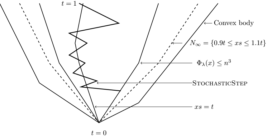
The key departure from the central path we present is that we can only maintain
\[0.9 t \leq \mu_i = x_{i}s_{i} \leq 1.1 t\]for some \(t>0\) instead of \(\mu\) close to \(t\) in \(\ell_2\) norm.
The short step central path proof maintains an invariant that \(\sum_{i}(x_{i}s_{i}-t)^{2}=O(t^{2})\). However, since our stochastic step has a stochastic noise with \(\ell_{2}\) norm as large as \(t\sqrt{\frac{n}{k}}\), one cannot hope to maintain \(x_{i}s_{i}\) close to \(t\) in \(\ell_{2}\) norm. Instead, we follow an idea in [LS14, LSW15] and maintain the following potential
\[\sum_{i=1}^{n}\cosh\left(\lambda\left(\frac{x_{i}s_{i}}{t}-1\right)\right)=n^{O(1)}\]with \(\lambda=\Theta(\log n)\). Note that the potential bounded by \(n^{O(1)}\) implies that \(x_{i}s_{i}\) is a multiplicative approximation of \(t\). We note that our algorithm is one of the very few central path algorithms [PRT02,M13,M16] that does not maintain \(x_i s_i\) close to some ideal vector in \(\ell_2\) norm. We are hopeful that our stochastic method and our proof will be useful for future research on interior point methods.
Projection Maintenance
The projection matrix we maintain is of the form \(\sqrt{W}A^{\top}\left(AWA^{\top}\right)^{-1}A\sqrt{W}\) where \(W=\mathrm{diag}(x/s)\). For intuition, we only explain how to maintain the matrix \(M_{w} := A^{\top}(AWA^{\top})^{-1}A\) for the short step central path step here. In this case, we have \(\sum_{i}\left(\frac{w_{i}^{\mathrm{new}}-w_{i}}{w_{i}}\right)^{2}=O(1)\) for each step.
If the changes of \(w\) is uniformly across all the coordinates, then \(w_{i}^{\mathrm{new}}=(1\pm\frac{1}{\sqrt{n}})w_{i}\) for all \(i\). Since it takes \(\sqrt{n}\) steps to change all coordinates by a constant factor and we only need to maintain \(M_{v}\) with \(v_{i}=\Theta(w_{i})\) for all \(i\), we can update the matrix every \(\sqrt{n}\) steps. Hence, the average cost of maintaining the projection matrix is \(n^{\omega-\frac{1}{2}}\), which is exactly what we desired.
For the other extreme case that the ‘‘adversary’’ puts all of his \(\ell_{2}\) budget on few coordinates, only \(\sqrt{n}\) coordinates are changed by a constant factor after \(\sqrt{n}\) iterations. In this case, instead of updating \(M_{w}\) every step, we can compute \(M_{w}h\) online by the woodbury matrix identity:
\[( M + U C V )^{-1} = M^{-1} - M^{-1} U ( C^{-1} + V M^{-1} U )^{-1} V M^{-1}.\]Let \(S \subset [n]\) denote the set of coordinates that is changed by more than a constant factor and \(r = |S|\). Using the identity above, we have the update rule
\[M_{w^{\mathrm{new}}} = M_{w} - (M_w)_S ( \Delta_{S,S}^{-1} + (M_w)_{S,S} )^{-1} ( (M_w)_S)^\top\]where \(\Delta=\mathrm{diag}(w^{\mathrm{new}}-w)\), \((M_w)_S\in \mathbb{R}^{n \times r}\) is the \(r\) columns from \(S\) of \(M_w\) and \((M_w)_{S,S},\Delta_{S,S} \in \mathbb{R}^{r \times r}\) are the \(r\) rows and columns from \(S\) of \(M_w\) and \(\Delta\).
As long as \(v_{i}=\Theta(w_{i})\) for all \(i\) except not too many coordinates, the update rule can be applied online efficiently. In another case, we can use the update rule instead to update the matrix \(M_{w}\) and the cost is dominated by multiplying a \(n\times n\) matrix with a \(n\times n^{r}\) matrix.
Since the cost of multiplying \(n\times n\) matrix by a \(n\times1\) matrix is same as the cost for \(n\times n\) with \(n\times n^{0.31}\) [GU18], the update rule should be used to update at least \(n^{0.31}\) coordinates. In the extreme case we are discussing, we only need to update the matrix \(n^{\frac{1}{2}-0.31}\) times and each takes \(n^{2}\) time, and hence the total cost is less than \(n^{\omega}\).
Epilogue
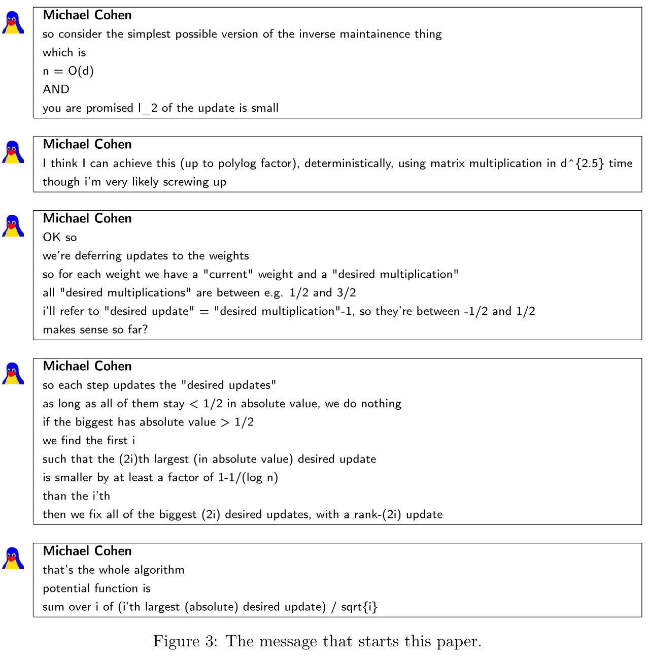
Since you have already read \(1/6\) of the paper, we encourage you to finish the whole paper. Finally, we want to say that we are honored and blessed to have collaborated with Michael Cohen. Arguably, this project is a simple corollary for his beautiful algorithm and proof for the inverse maintenance problem, described in the the following figure. We believe that his enthusiasm in finding the proofs from The Book will be remembered.