


Introduction
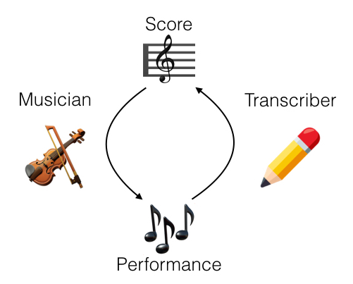
The production of classical western music is a two stage process. First a composer writes down a score: written notation that indicates a particular musical structure. Then a performer reads this score and manipulates an instrument as indicated by the score to produce audio waves that a human ear perceives as music. A trained musician is also capable of transcribing a performance: while listening to a musical performance, the musician can write down the score that the performer used to guide the performance.

Figure 1. A musician creates a musical performance from a score. A performance can be transcribed by a musician to recover the score.
The closed loop in this figure implies that the musician and transcription channels are lossless. Indeed, for western classical music this is mostly the case: performers are expected to render a faithful performance of the score provided to them, and so it is possible for the transcriber to precisely recover the original score.1 In this post, we will consider methods that replace the human transcriber in this loop with an automated algorithm.
Notation
Let \(\mathcal{S}\) denote the space of scores and \(\mathcal{P}\) the space of performances. We will write \(f : \mathcal{S} \to \mathcal{P}\) to indicate a performance of a score (\(f\) will be random, to account for variability in the performance of a particular score). We want to find an inverse function \(f^{-1} : \mathcal{P} \to \mathcal{S}\) such that \(f^{-1} \circ f (s) = s\) for all \(s \in \mathcal{S}\).
Specifically, we will represent a score as a binary indicator matrix \(s \in \{0,1\}^{T \times N}\), where \(T\) is the length of the score (discretized at some rate) and \(N\) is the range of possible notes (e.g. \(88\) piano keys). We can represent a performance with air pressure variation measurements captured by a microphone; these measurements are typically sampled at a rate of \(44.1kHz\), so a performance of length \(T\) can be represented by a vector \(p \in \mathbb{R}^{T\times 44100}\). One way to formulate our problem is to ask for a function \(f^{-1} : \mathbb{R}^{T\times 44100} \to \{0,1\}^{T \times N}\) such that \(f^{-1}\circ f(s) = s\) for all \(s \in \mathcal{S}\).
This formulation has some major flaws. First, it is extremely highly dimensional. Second, it only works for scores of length \(T\); if we encounter a score of some other length, our function is undefined and we cannot transcribe it. What we really want is a function \(f^{-1} : \mathbb{R}^{c \times 44100} \to \{0,1\}^N\) that predicts which notes are on at a particular time \(t \in [0,T)\) given a local vector of contextual audio surrounding time \(t\) (in practice \(c = .5\), a half second of context, is usually reasonable). To transcribe a recording and construct a full \(T \times N\) dimensional score, we can simply slide our frame predictor along from the beginning to the end of the audio, writing down the notes at each time point.
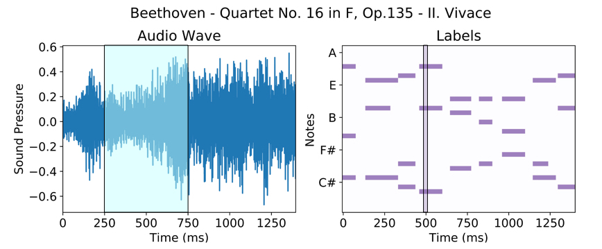
Figure 2. (Left) Audio recording, with highlighted half-second frame of context for prediction of notes at time \(500\) ms. (Right) Score with highlighted note-vector that we wish to predict.
Historical highlights
Transcription methods based on fourier analysis were proposed as early as the 1970s by Piszczalski and Galler (1977). The machine learning community took an interest in this problem beginning with Raphael (2002). Early work on this problem from a learning perspective was stymied by the difficulty of obtaining labels on an audio sequence. A score on its own is insufficient in two ways. First, it must be digitized: a pdf score cannot be easily converted to a binary matrix format. Second, it must be aligned to a recording: a score describes the sequence and relative timings of events in a performance, but the performer decides:
-
When the performance will begin.
-
The speed of the performance (within bounds set by the composer).
-
Deliberate deviations from this speed for emotional effect.
-
Random fluctuations in the speed due to human fallibility.
Each of these problems is daunting, so early work focused on unsupervised methods (Raphael’s work fits an HMM with Baum-Welch).
To the best of my knowledge, music transcription was first considered as a supervised learning problem by Poliner and Ellis (2006). These researchers surmounted the digitization problem by leveraging a growing body of MIDI files, produced by a community of enthusiasts, which encode much of the information of a score in a parsable digital format. They surmounted the alignment problem by producing their own performances using music synthesis software. By constructing artificial performances, they were able to exert precise control over timings in the resulting audio and exactly align their MIDIs to the audio.
Recent developments
Within the supervised transcription framework introduced in Poliner and Ellis, there are at least three avenues for performance improvements. First, models trained on synthesized performances may not generalize well to human performances so we may want to construct a better dataset. Second, the model introduced by Poliner and Ellis is a standard SVM on magnitude spectrum features; it may be possible to construct a better acoustic model, tailored with prior information about the structure of music. Third, the frame-based framework doesn’t capture the (rich) time-series structure of the label space: each frame is predicted independently.
Datasets. The easiest way to solve the domain adaptation problem is to eliminate it by finding some way to align human performances to scores. A solution to this problem was proposed in an earlier paper by Ellis himself (Turetsky and Ellis, 2003). We discuss MusicNet below, which was constructed using a variant of Ellis’s technique. As of 2018, many datasets of music-aligned scores are available for various genres:
-
Sync-RWC. Goto, Hashiguchi, Nishimura, and Oka (2003).
-
MAPS. Emiya, Badeau, and David (2010).
-
Lakh. Raffel (2016).
-
MusicNet. Thickstun, Harchaoui, and Kakade (2017).
Acoustic models. Neural acoustic models have become popular in recent years. Several research teams have proposed deep acoustic models for transcription: see Nam, Ngiam, Lee, and Slaney (2011) as well as Trabelsi, Bilaniuk, Serdyuk, Subramanian, Santos, Mehri, Rostamzadeh, Bengio, and Pal (2018). There has also been interest in applying convolutional ideas to transcription: Bittner, McFee, Salamon, Li, and Bello (2017), as well as Pons and Serra (2017). Our own work at University of Washington (discussed below) also pursues some of these convolutional ideas: Thickstun, Harchaoui, and Kakade (2017) and Thickstun, Harchaoui, Foster, and Kakade (2018).
Time series. Some recent work breaks away from the strict frame-based task and seeks to incorporate time-series structure in the label space of scores to improve transcriptions. These methods typically combine a frame-based acoustic model with a recurrent state-space model. See Sigtia, Benetos, Boulanger-Lewandowski, Weyde, Garcez, and Dixon (2015) as well as Sigtia, Benetos, and Dixon (2016). These ideas are crucially important to achieving the best performance on this task, but they are somewhat orthogonal to the acoustic modeling concerns and we won’t consider them in this post.
Music-to-score alignment
To align a performance to a score, we need an observation and a key idea. The observation is that if a performance and score are aligned, then at each time location \(t\) the vector of notes in the score \(s_t \in \{0,1\}^{128}\) and the local frame of audio \(X_t \in \mathbb{R}^{c\times 44100}\) will be “similar,” in the sense of a cost \(C\) that we will make precise shortly. The key idea is to minimize the total dissimilarity at each point \(t \in [0,T)\) between \(X_t\) and \(s_t\). We do this by shrinking or stretching the performance \(X \in \mathcal{P}\), resulting in a minimal-cost alignment between the performance and the score.
Mathematically, this shrinking and stretching amounts to solving the following optimization problem (\(X_{t_i} \in \mathbb{R}^{c\times 44100}\) indicates the local contextual frame of audio in the performance \(X\) centered around time \(t_i\)):
\[\begin{array}{ll@{}ll} \underset{t \in \mathbb{N}^T}{\text{minimize}} & \displaystyle\sum_{i=1}^n C(X_{t_i},s_i)&\\ \text{subject to}& t_0 = 0, & \\ & t_n = m, & \\ & t_i \leq t_j & \text{if $i < j$}. & \end{array}\]Dynamic time warping gives an exact solution to this problem in \(\mathcal{O}(mn)\) time and space, where \(m\) is the length of the performance and \(n\) is the length of the score.
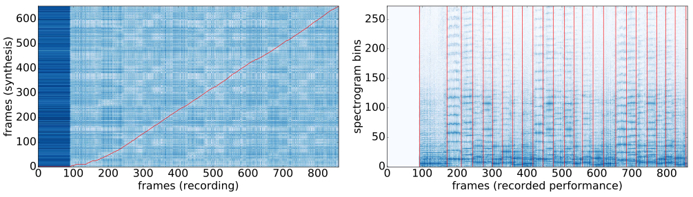
Figure 3. (Left) A heatmap of local alignment costs between the synthesized and recorded spectrograms, with the optimal alignment path in red. The block from \(x = 0\) to \(x = 100\) frames corresponds to silence at the beginning of the recorded performance. The slope of the alignment can be interpreted as an instantaneous tempo ratio between the recorded and synthesized performances. The curvature in the alignment between \(x = 100\) and \(x = 175\) corresponds to an extension of the first notes by the performer. (Right) Annotation of note onsets on the spectrogram of the recorded performance, determined by the alignment shown on the left.
The success of dynamic time warping depends crucially on defining a good cost metric; i.e. a cost that is small at points where \(X\) and \(s\) are well-aligned. This is complicated by the fact that points \(X_{t_i}\) and \(s_i\) do not even live in the same space. The clever idea introduced by Turetsky and Ellis (2003) is to map the score \(s\) into performance-space by synthesizing it. Now we have two vectors \(X_t\) and \(\text{Synth}(s_i)\) in \(\mathbb{R}^{c\times 44100}\) and we can compare them using standard metrics (e.g. \(L^p\) metrics). Actually, we need to be a little more clever than this; we really want our comparisons to be phase-invariant, so we will actually further transform each of our vectors into the fourier domain and compare their magnitude spectra.
We can and have applied this automated alignment procedure to construct a large dataset of labeled classical music. MusicNet is available here. For further information about the construction and contents of MusicNet, see Thickstun, Harchaoui, and Kakade (2017).
Translation-invariant networks
Prepared with a large dataset of labeled human performances, we can turn our attention to models that efficiently capture the structure between the performances and labels. While we can produce a large dataset using automated alignments, it is necessarily finite. This stands in contrast with synthesized datasets, which can be configured to generate an effectively infinite stream of artificial performances. Therefore we will focus on models that efficiently capture correlations in our data. Keeping the bias-variance tradeoff in mind, we will bias our model using prior information about music.
In particular, we will exploit a translation-invariance in music using a convolutional architecture. Consider, for motivation, a major triad chord. The concept of a major chord is preserved under translations in log-frequency space. If we learn convolutional filters over the log-frequency domain, we can capture the concept of a major triad using a single filter. Contrast this situation to a fully connected layer over log-frequencies, which would need to learn this pattern many times over, once for each root position of the chord. Therefore, our first step will be to pre-process our data by mapping it into a log-frequency domain. We will then convolve along the frequency axis of our filterbank to capture frequency-invariant features of our data.
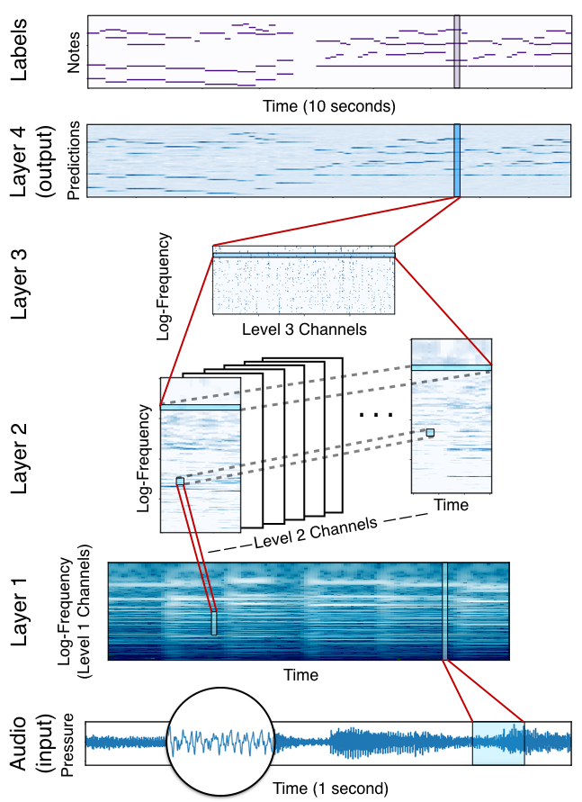
Figure 4. A translation-invariant network for note classification. Audio input maps to Layer 1 according to the log-spaced, cosine-windowed filterbank. Layer 1 maps to Layer 2 by convolving a set of \(128 \times 1\) learned filters along the log-frequency axis at each fixed time location. Layer 2 maps to Layer 3 by convolving again along the log-frequency axis, this time with a set of filters of height 1 that fully connect along the time and channel axes of Layer 2. Notes are predicted at Layer 4 by linear classification on the Layer 3 representation.
Further exploiting our awareness of frequency-invariance, we augment our data by stretching or shrinking our input audio with linear interpolation. This corresponds to a pitch-shift in the frequency domain. For small shifts (\(\pm 5\) semitones or less) the transformed audio sounds natural to the human ear. Randomly shifting each data point in a minibatch by an integral number of semitones in the range \([-5, 5]\) augments the dataset by an order of magnitude. And the translational nature of this augmentation reinforces the architectural structure of the translation-invariant network. In addition to an integral semitone shift, we also apply a continuous shift to each data point in the range \([-.1, .1]\). This makes the models more robust to tuning variation between recordings.
Last year we submitted this translation-invariant model to the MIREX Multiple Fundamental Frequency Estimation challenge. This is a frame-based transcription task based on the Poliner and Ellis framework discussed in this blog post. Table 1 summarizes results for the top 5 participants in 2017. THK1 is the translation-invariant model described in this section. For further information about the translation-invariant network architecture see Thickstun, Harchaoui, Foster, and Kakade (2018).
| Model | Precision | Recall | Accuracy | Etot |
| MIREX 2009 Dataset: | ||||
|---|---|---|---|---|
| THK1 | 82.2 | 78.9 | 72.0 | .316 |
| KD1 | 72.4 | 81.1 | 66.9 | .419 |
| MHMTM1 | 72.7 | 78.2 | 65.5 | .441 |
| WCS1 | 64.0 | 80.6 | 59.3 | .569 |
| ZCY2 | 62.7 | 56.2 | 50.6 | .601 |
| Su Dataset: | ||||
| THK1 | 70.1 | 54.6 | 51.0 | .529 |
| KD1 | 45.9 | 45.0 | 38.1 | .745 |
| WCS1 | 63.6 | 39.7 | 35.7 | .700 |
| MHMTM1 | 61.2 | 36.8 | 35.2 | .676 |
| ZCY2 | 40.9 | 28.2 | 26.2 | .799 |
Table 1. MIREX 2017 transcription results. Models are evaluated on two datasets, the MIREX 2009 dataset and the Su dataset. For details, see here.
References
Martin Piszczalski and Bernard A. Galler. 1977. “Automatic music transcription.” Computer Music Journal, Vol. 1, No. 4, pp. 24-31. https://www.jstor.org/stable/40731297
Christopher Raphael. 2002. “Automatic transcription of piano music.” Proceedings of the International Society of Music Information Retrieval. http://www.ismir2002.ismir.net/proceedings/02-FP01-2.pdf
Graham E. Poliner and Daniel P. W. Ellis. 2006. “A discriminative model for polyphonic piano transcription.” EURASIP Journal on Applied Signal Processing. https://link.springer.com/content/pdf/10.1155/2007/48317.pdf
Robert J. Turetsky and Daniel P. W. Ellis. 2003. “Ground-truth transcriptions of real music from force-aligned midi syntheses.” https://jscholarship.library.jhu.edu/bitstream/handle/1774.2/20/paper.pdf
Masataka Goto, Hiroki Hashiguchi, Takuichi Nishimura, and Ryuichi Oka.2003. “RWC music database: Music genre database and musical instrument sound database.” https://jscholarship.library.jhu.edu/bitstream/handle/1774.2/36/paper.pdf
Colin Raffel. 2016. “Learning-based methods for comparing sequences, with applications to audio-to-midi alignment and matching.” PhD Thesis. http://colinraffel.com/publications/thesis.pdf
Juhan Nam, Jiquan Ngiam, Honglak Lee, and Malcolm Slaney. 2011. “A Classification-Based Polyphonic Piano Transcription Approach Using Learned Feature Representations.” International Society of Music Information Retrieval, pp. 175-180. https://www-cs.stanford.edu/~jngiam/papers/ismir2011-PolyphonicTranscription.pdf
Chiheb Trabelsi, Olexa Bilaniuk, Dmitriy Serdyuk, Sandeep Subramanian, João Felipe Santos, Soroush Mehri, Negar Rostamzadeh, Yoshua Bengio, and Christopher J. Pal. 2018. “Deep complex networks.” International Conference on Learning Representations. https://arxiv.org/pdf/1705.09792.pdf
Rachel M. Bittner, Brian McFee, Justin Salamon, Peter Li, and Juan P. Bello. 2017. “Deep salience representations for f0 estimation in polyphonic music.” International Society for Music Information Retrieval Conference, Suzhou, China, pp. 23-27. http://www.justinsalamon.com/uploads/4/3/9/4/4394963/bittner_deepsalience_ismir_2017.pdf
Jordi Pons and Xavier Serra. 2017. “Designing efficient architectures for modeling temporal features with convolutional neural networks.” In IEEE International Conference on Acoustics, Speech and Signal Processing, pp. 2472-2476. http://jordipons.me/media/PonsSerraICASSP2017.pdf
John Thickstun, Zaid Harchaoui, and Sham M. Kakade. 2017. “Learning features of music from scratch.” In International Conference on Learning Representations. https://arxiv.org/pdf/1611.09827.pdf
John Thickstun, Zaid Harchaoui, Dean P. Foster, and Sham M. Kakade. 2018. “Invariances and data augmentation for supervised music transcription.” In IEEE International Conference on Acoustics, Speech, and Signal Processing. https://arxiv.org/abs/1711.04845
Siddharth Sigtia, Emmanouil Benetos, Nicolas Boulanger-Lewandowski, Tillman Weyde, Artur S. d’Avila Garcez, and Simon Dixon. 2015. “A hybrid recurrent neural network for music transcription.” In IEEE International Conference on Acoustics, Speech and Signal Processing, pp. 2061-2065. https://arxiv.org/pdf/1411.1623.pdf
Siddharth Sigtia, Emmanouil Benetos, and Simon Dixon. 2016. “An end-to-end neural network for polyphonic piano music transcription.” IEEE Transactions on Audio, Speech and Language Processing 24, no. 5. http://ieeexplore.ieee.org/abstract/document/7416164/
-
This would not be true of other genres, jazz for example. ↩