
This blog post decribes the recent NeurIPS 2018 paper and companion code on smooth training of max-margin structured prediction models. Training structured prediction models consists in optimizing a non-smooth objective using an inference combinatorial optimization algorithm.
We propose a framework called Casimir based on the Catalyst acceleration and infimal-convolution smoothing allowing us to break the non-smoothness barrier and obtain fast incremental algorithms for large-scale training of deep structured prediction models.
Setting
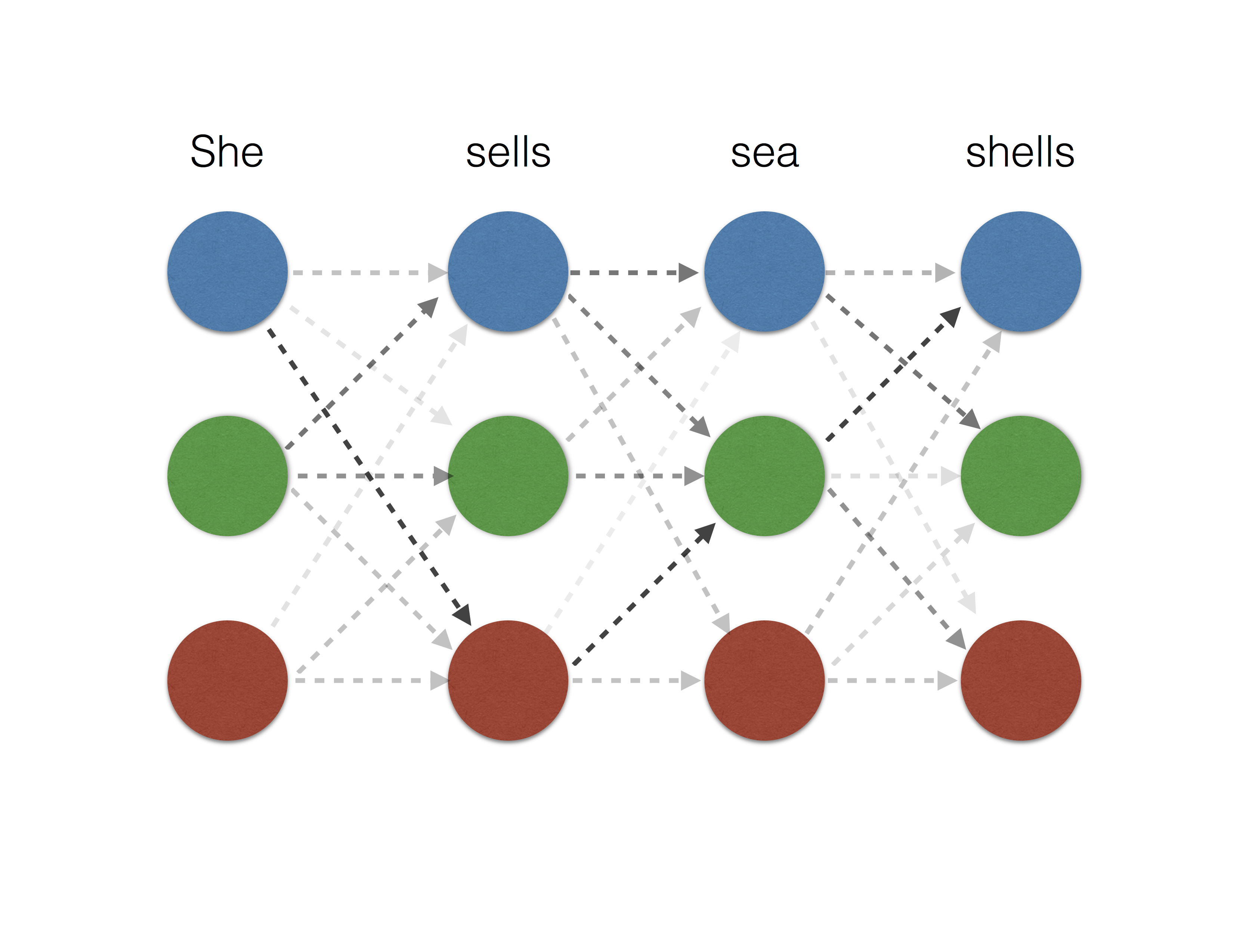
Structured prediction consists in predicting complex outputs such as sequences, trees or lattices. For instance, named entity recognition can be cast as the task of predicting a sequence of tags, one for each word which identifies the word as a named entity.

In this example, an output is a chain of tags, where each tag can take values from a dictionary. In general, the set \(\mathcal{Y}\) of all outputs is finite but too large to enumerate. To overcome this difficulty, a score function \(\phi(\cdot, \cdot; w)\), parameterized by \(w\), is defined to measure the compatibility of the input-output pair \((x, y)\) as \(\phi(x,y;w)\). This score function decomposes over the structure of the outputs (e.g., a chain) so that predictions can be made by an inference procedure which finds
\[y^*(x ; w) \in \operatorname*{arg max}_{y \in \mathcal{Y}} \phi(x, y ; w) \,.\]The inference problem can be solved in various settings of interest by efficient combinatorial algorithms such as the Viterbi algorithm for named entity recognition.
The goal of the learning problem is to find the best parameter \(w\) so that inference \(y^*(x ; w)\) produces the correct output. Given a loss \(\ell\) such as the Hamming loss, max-margin structured prediction aims to minimize a surrogate called the structural hinge loss, which is defined for an input-output pair \((x_i, y_i)\) as
\[f_i(w) = \max_{y \in \mathcal{Y}} \psi_i(y; w) \,,\]where \(\psi_i\) is defined as a generalization of the margin used in classical support vector machine,
\[\psi_i(y; w) = \phi(x_i, y ; w) + \ell(y_i, y) - \phi(x_i, y_i ; w) \,.\]The optimization problem is defined for samples \(\{(x_i, y_i)\}_{i=1}^n\) as the regularized empirical surrogate risk minimization
\[\min_w \left[ F(w) = \frac{1}{n}\sum_{i=1}^n f_i(w) + \frac{\lambda}{2}\|w\|_2^2 \right] \,.\]The subgradient of \(f_i\) is computed by running the inference procedure as
\[\partial f_i(w) \in \operatorname*{arg max}_{y \in \mathcal{Y}} \psi_i(y ; w) \,.\]Though the above formulation allows one to use tractable first-order information through combinatorial procedures, its non-smoothness prevents us from using fast incremental optimization algorithms. We overcome this challenge by blending an extrapolation scheme for acceleration and an adaptive smoothing scheme.
Smoothing
We now wish to smooth the objective function \(F\) in order to apply incremental algorithms for smooth optimization. This is not straightforward because each \(f_i\) is computed by a discrete inference algorithms.
To smooth \(f_i\), we first note that it can be written as the composition \(f_i = h \circ g_i\), where
\[g_i(w) = \big(\psi_i(y;w) \big)_{y \in \mathcal{Y}} \,, \quad \text{and} \quad h(z) = \max_{i \in |\mathcal{Y}|} z_i.\]The non-smooth max function \(h\) is simply smoothed by adding a strongly convex function \(\omega\) to its dual formulation as
\[h_{\mu\omega}(w) = \max_{u \in \Delta^{|\mathcal{Y}|}} \{ z^\top u - \mu \omega(u) \} \,,\]where \(\Delta^m\) is the simplex in \(\mathbb{R}^m\). It can be shown that \(h_{\mu\omega}\) is a smooth approximation of \(h\) upto \(O(\mu)\) [N05,BT12]. Common choices of \(\omega\) are given below.
| Smoothing type | \(\omega(u)\) | Smoothing computation |
|---|---|---|
| entropy | \(H(u) = \langle u, \log u \rangle\) | log-sum-exp |
| \(\ell_2^2\) | \(\ell_2^2(u) = \tfrac{1}{2}|u|^2_2\) | projection on simplex |
The smooth structural hinge loss is obtained by replacing the non-smooth \(h\) with its smooth counterpart as
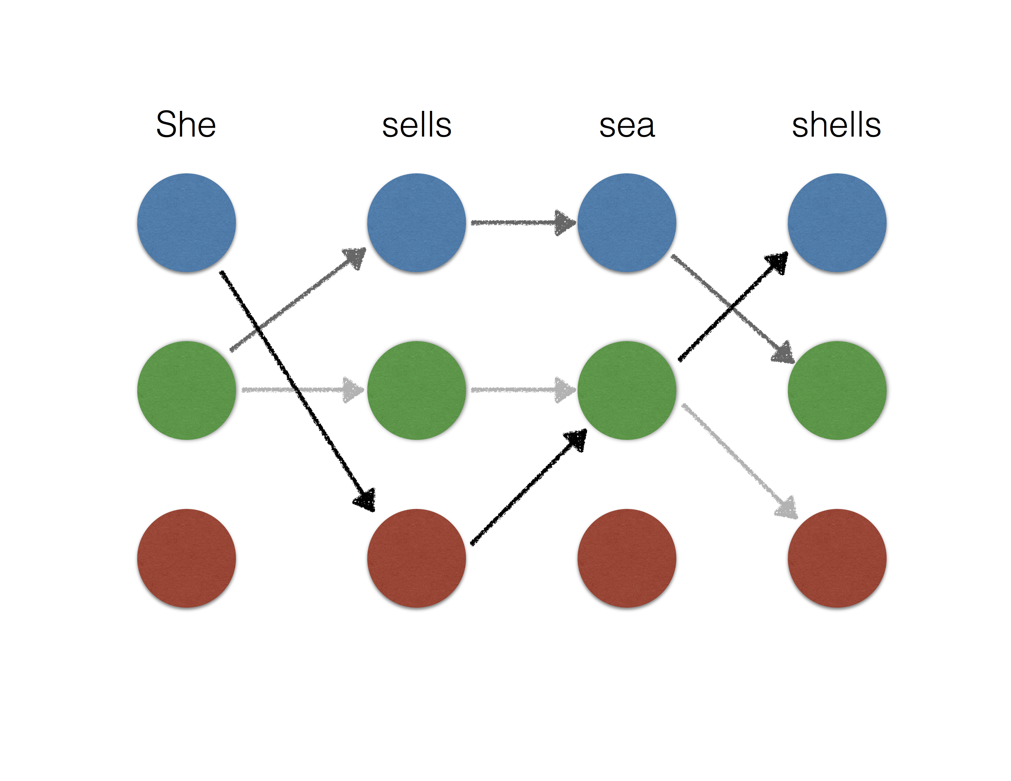
\[f_{i, \mu \omega} = h_{\mu\omega} \circ g_i.\]In the structured prediction setting, entropy smoothing is equivalent to a conditional random field [LMP01], which is only tractable for tree structured outputs. On the other hand, the sparse outputs of \(\ell_2^2\) smoothing can be well approximated by picking a small integer \(K\) and considering the top-\(K\) highest scoring outputs. This makes \(\ell_2^2\) smoothing more feasible for tree structured outputs as well as select loopy output structures. See the illustration below for the example of named entity recognition.
 |
 |
 |
|---|---|---|
| Non-smooth | \(\ell_2^2\) smoothing | entropy smoothing |
Formally, we define inference oracles, namely the max, top-\(K\) and exp oracles as first order oracles for the structural hinge loss and its smoothed variants with \(\ell_2^2\) and entropy smoothing respectively. This allows us to measure the complexity of optimization algorithms, which we discuss next. The table below shows how the smooth inference oracles are implemented for a given max oracle. Their computational complexity is given in terms of \(\mathcal{T}\), the cost of max oracle and \(p\), the size of each output \(y\).
| Max oracle | Top-\(K\) oracle | Exp oracle |
|---|---|---|
| Max-product | Top-\(K\) max-product, \(\widetilde O(K\mathcal{T})\) time | Sum-product, \(O(\mathcal{T})\) time |
| Graph cut | BMMF, \(O(pK \mathcal{T})\) time | Intractable |
| Graph matching | BMMF, \(O(K \mathcal{T})\) time | Intractable |
| Branch and bound search | Top-\(K\) search | Intractable |
Here, BMMF is the Best max marginal first algorithm of [YW03].
Optimization algorithms
The optimization algorithms depend on the nature of the map \(w \mapsto \phi(x, y ; w)\). The structural hinge loss, and thus \(F\), are convex if this map is linear. Otherwise, \(F\) could be nonconvex in general.
Convex structured prediction
Classical structured prediction [ATH03, TGK04] uses a linear score \(\phi(x, y;w)=w^\top \Phi(x, y)\) where \(\Phi(x, y)\) is a hand-engineered feature map. The objective \(F\) is convex here and we extend the generic Catalyst acceleration scheme [LMH18] to optimize nonsmooth objectives by using smooth surrogates. See also this blog post for a review. In particular, each iteration considers smoothed and regularized surrogates of the form
\[F_{\mu, \kappa}(w ; z) = \frac{1}{n}\sum_{i=1}^n f_{i, \mu}(w) + \frac{\lambda}{2}\|w\|^2_2 + \frac{\kappa}{2}\|w-z\|^2_2 \,.\]Algorithm
Starting at \(z_0 = w_0\), at each step \(k\), do
- Approximately solve using a linearly convergent algorithm \(\mathcal{M}\):
- Extrapolate to get
When using, for instance, SVRG [JZ15] as the linearly convergent algorithm \(\mathcal{M}\), we are guaranteed to get approximate solution \(F(w_k)-F^* \leq \epsilon\) after \(N\) iterations where
\[\mathbb{E}(N) = \begin{cases} O \left(n + \sqrt{\frac{n}{\lambda \epsilon}} \right), \quad \mbox{if fixed smoothing}\\ O \left(n + {\frac{1}{\lambda \epsilon}} \right), \quad \mbox{if adaptive smoothing} \end{cases}\]Deep structured prediction
More broadly, deep structured prediction attempts to learn the feature map \(\Phi\). The score function \(\phi(x, y ; w) = w_2^\top \Phi(x, y; w_1)\) is nonlinear in \(w = (w_1, w_2)\) so that \(F\) is nonconvex. In this case, the prox-linear algorithm [B85,DP18] is applicable. It was described previously here. This amounts to considering a linear approximation to \(\psi\) as
\[\psi_i(y ; w, z) = \psi_i(y ; z) + \nabla_z \psi_i(y ; z)(w-z) \quad \text{and} \quad f_i(w ; z) = \max_{y \in \mathcal{Y}} \psi_i(y ; w, z) \,,\]to get a regularized convex model
\[F_\gamma(w ; z) = \frac{1}{n}\sum_{i=1}^n f_i(w ; z) + \frac{\lambda}{2}\|w\|_2^2 + \frac{1}{2\gamma} \|w-z\|_2^2 \,.\]The convex sub-problem above can then be optimized by the convex optimization algorithm described earlier.
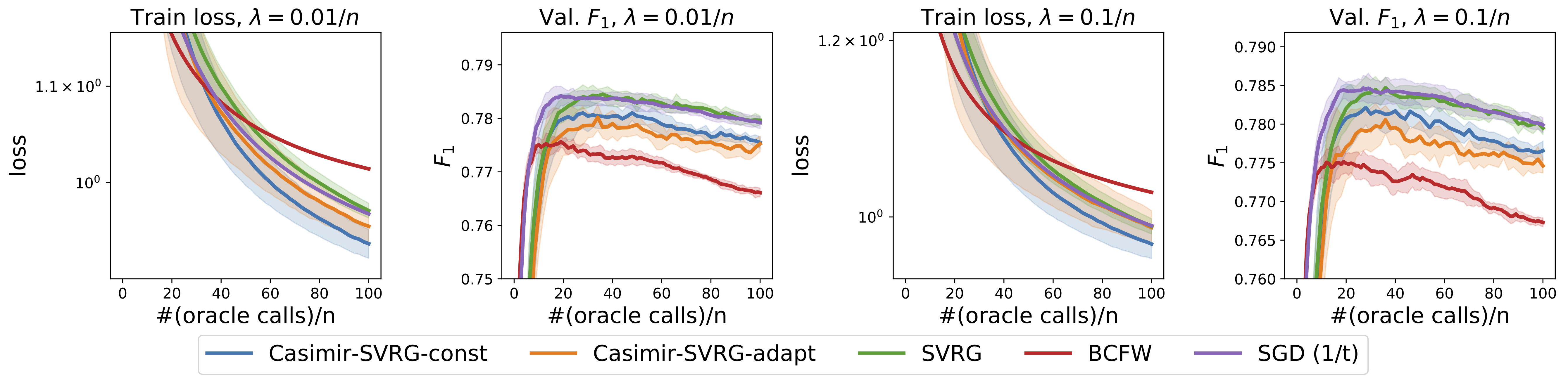
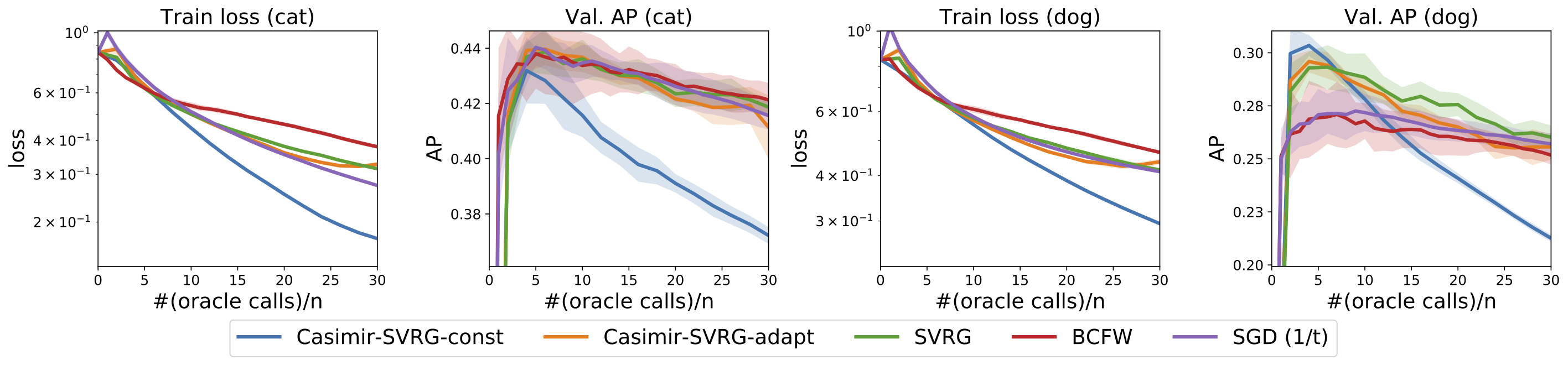
Numerical experiments
Given below are results of numerical experiments for named entity recognition on CoNLL-2003 dataset and visual object localization on the PASCAL VOC dataset. We first show the performance of the proposed algorithm for the convex case, where the feature maps are predefined. Casimir-SVRG-const and Casimir-SVRG-adapt are the two variants with constant and adaptive smoothing respectively.
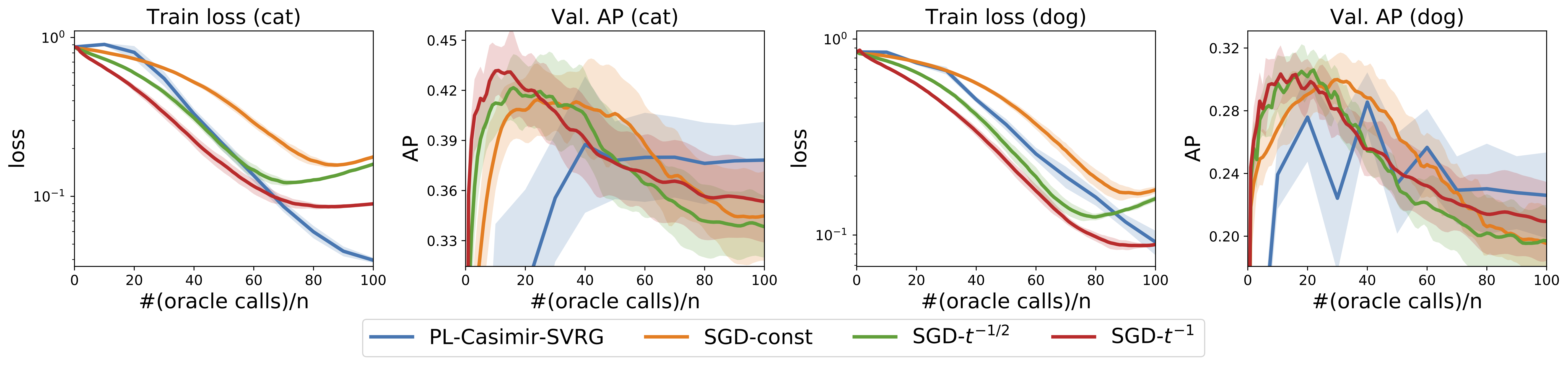
Next, we consider deep structured prediction where the feature map is learnt using a convolutional neural network.
A software package called Casimir implementing all these algorithms and more is available here.